Properties FAQ
Back to Top
How can I calculate polarizability?
Spartan can calculate polarizability in 4 ways:
- Using the empirical formula described
below. This available in the QSAR tab of the properties
panel and
is available for all quantum mechanical levels. (It can be
displayed in the spreadsheet with the
"Polarizability=@PROP(EST_POLARIZ)"
function).
- The polarizability can be calculated from first principles
with the addition of the POLAR keyword.
For information on how to get frequency dependent
polarizability see the POLAR= keyword
in the keywords section of this FAQ. A summary of this
calculation is printed in the output file. For more detail
you can use the
KEEPVERBOSE keyword
-
An external (multipole) field can be applied to any calculation
and the dipole can be compared with the original value.
As an example one could use
EMFIELD=X~0.01
keyword with an Energy calculation
then use the
spreadsheet equation
=(1/2.542)*(@ref(@row-1,@prop(dipole_vec,1))-@prop(dipole_vec,1))/.01
to calculate the x component of the polarizability.
(The "@row-1" assumes the molecule immediately preceding the polarized
molecule has the same coordinates and method, but without the applied field.
- When using semi-empirical methods the polarizability can be
calculated with the POLAR keyword.
For HF calculations this keyword also calculates the
hyperpolarizability using the
method described by Kurtz in
H.A. Kurtz et. al., J. Comp. Chem., 11, 82, 1990.
Both the polarizability and
hyperpolarizability tensors are provided as well as the experimentally
observed
'average polarizability' (alpha),
the 'first hyperpolarizability' (beta), and
the 'mean second hyperpolarizability' (gamma).
These values are printed in the output. It should be noted
that in the output two different equations are used to
calculate polarizabilities. (E4 is the energy equations
and 'dip' is the dipole equation--from the Kurtz paper.)
The main difference between these methods is sensitivity
to 'round off' error. The difference can be used as an
estimate of the uncertainty in the final results.
Note that the details are in the verbose output, so make
sure to use the KEEPVERBOSE keyword or set the
"Keep Verbose" option in the "Preferences Dialog".
These values are accessible from the spreadsheet with the
@PROP() possible options are:
- POLAR_STATIC_ALPHA
- POLAR_STATIC_BETA
- POLAR_STATIC_GAMMA
- POLAR_STATIC_TENSOR
- POLAR2_STATIC_TENSOR (18 elements).
Back to Top
What are the units of polarizability?
Polarizability calculated in the properties module is derived
from an empirical formula:
  electronegativity:      -( E_HOMO + E_LUMO )/2
  hardness         :      -( E_HOMO - E_LUMO )/2
  polarizability    : 0.08 * VdW_Volume
                     -13.0352*hardness + 0.979920*hardness^2
                     +41.3791
    The final units are in
      10-30 m3
Electron Densities, Spin Densities, Dipole Moments, Charges
and Electrostatic Potentials
To get the more traditional units of coul2*m/N
we divide by the permittivity of free space (and 4*π)
and then scale to units appropriate for the atomic scale.
To convert from "au" (as calculated by the quantum calculations)
to coul2m/N (or coul2m2/J) one must multiply by
[1/bohr]3*[4*πεo] =
[0.148185x10⁻³⁰]*[ 111.21x10⁻¹² ] = 16.4877x10-42
      1 a.u. = 16.4877x10-42 coul2*m/N
      1 a.u. =  0.148185 A3
      1 a.u. =  0.148185 m-30
      1 a.u. =  0.373803244 cm3/mol
      1 a.u. = (1/2.542) D (used in the numerical calculation)
For example an HF/6-31+G(2df) calculation of carbon monoxide gives
polarizability of "10" in the direction perpendicular to the
molecular axis, which is
1.65x10-40 coul2m/N, in fair agreement
with experiment (2+-0.5).
Where do the terms of the empirical polarizability formula come from?
Though these
coefficients may appear arbitrary, the first term
is derived from an estimation that assumes all atoms have the
polarizability of hydrogen,
with a correction applied from the energy gap of the highest occupied &
lowest unoccupied molecular orbitals. This equation is only used in the
semi-empirical methods--and it turns out that this is a fairly good
first guess. From a freshman physics textbook, the answer should
be (for atomic groups):
     H    0.66
     He   0.21
     Li  12
     Be   9.3
     C    1.5
     Ne   0.4
     Na  27
     Ar   1.6
     K   34
Back to Top
What are Q-plus and Q-minus?
Q-plus is the largest positive charge on hydrogens.
Q-minus is the largest negative charge.
Q-plus & Q-minus are known as the 'TLSER' parameters.
Back to Top
What is ovality and how is it calculated?
Ovality is a measure of how the shape of the molecule approaches a sphere or cigar.
Ovality is described by the ratio of volume and area:
    O = A/(4*pi*((3*V)/4*pi)^(2/3))
      where
        A : Area
        V : Volume
        O : Ovality
Thus the He atom is 1.0 and HC24H (12 triple
bonds) is ~1.7.
Back to Top
What are electronegativity and hardness?
The molecular electronegativity and hardness are generalizations of the
same concept at the atomic level:
| electronegativity | = -(HOMO + LUMO)/2 |
| hardness | = -(HOMO - LUMO)/2 |
Back to Top
How are the volume and surface area calculated?
In the QSAR panel of the "Molecule Properties"
dialog we show a few volume/area related properties,
and these fall into two categories:
"From CPK Model" and "From Electron Density".
- From CPK Model: These are calcualted analytically
from Spartan's default
VdW radii for each atom.
These can be seen and modified via the
Preference dialog.
Wavefunction's default VdW values are a collection of radii
coming from Bondi's original paper
○ Bondi, J PC 68 (1964) 441
With modification from
○ Charton, Motoc, "Steric Effect in Drug Design" Springer-Verlag, p.62
and the remaining atoms by scaling (by 0.90) UFF VdW radii
○ "a Full Periodic Table Force Field", J. Am. CHem. Soc. Vol. 114, 24 (1992) 10035
- From Electron Density: When the "QSAR" check-box
is selected in the Calculations dialog the surface area
and volume calcualted using 0.002 e/au3
iso-density plot of the electron density plot.
The exposed atom area display in the "Atom Properties" dialog is calculated
using the CPK Model.
Back to Top
What "logP" models does Spartan provide?
- The Villar method is available from
semi-empirical calculations (with no d-orbitals). The Villar method
examines the overlap matrix, searching for
the type and number of lone pairs as well as the surface
area of each atom; it is parameterized for H,C,N,O,F,S,Cl.
The reference is:
- Ibon Alkorta, Hugo O. Villar,
Int. J. Quant. Chem. Vol. 44, 203-218 (1992)
- Angelina Kantola, Hugo O. Villar, Gilda H. Loew,
J. Comp. Chem. vol. 12, No. 6, 681-689 (1991)
- Ghose-Crippen is Spartan's default method for calculating
logP. This method is independent of the
energy/wavefunction. (i.e. one will get the same results from mechanics,
semi-empirical, HF, DFT, and MP2 calculations). However, the Ghose-Crippen method is dependent on how
the molecule is drawn/connected. The Ghose-Crippen method
is parameterized for
110 atom/bonding types, including common bondings of H,C,N,O,S and
the Halogens.
For a test suite of 494 compounds, it provides a standard deviation of
.347 and correlated coefficient of .962.
In a test suite of 69 compounds beyond the original test suite
it predicts a variance of .404.
The reference is:
- Ghose, Pritchett and Crippen J. Comput. Chem., 9, 80 (1988)
- LogP can also be calculated directly from solvation energy.
For example one can run a calculation with the
POSTSOLVENT=SM8:1OCTANOL and then
POSTSOLVENT=SM8:WATER keywords and use those energies in the
equation
LogP = [ SolvEwater - SolvE1-octanol ] / 5.707
(all energies in kJ/mol; the 5.707 is log(10)*RT )
The solvation energy is printed in the output, or can be put into the spreadsheet
by putting the following equation into a column header:
SolvE = @energySolv*@hart2kj
"logP" methods can be selected with the LOGP= keyword;
LOGP=VILLAR and LOGP=GHOSE
respectively.
An example Spartan file shows some of these
logP examples on a broad range of simple molecules. While one can argue
over which of these calculations is most precise or efficient, the noise
in all these methods is typically smaller than the uncertainty in using
LogP to predict common properties like blood/brain barriers.
Back to Top
What solvation models does Spartan provide?
Spartan includes a number of ways to examine solvation.
- C-PCM
The default solvation model which we advise for geometry and
frequency calculations is the C-PCM model
(Conductor like Polarizable continuum model).
This depends on the shape and charge distribution of the
molecule (solute) and the dielectric of the solvent.
Continuum models such as C-PCM do not account for explicit
solvent-solute interactions such as hydrogen bonding or
'explicit hydrophobic'. For this reason we do not report an
"energy of solvation".
Spartan gives easy access to three different dielectrics:
"NonPolar" (7.43 same as THF),
"Polar" (37.22, same as dimethylformamide),
and "Water" (78.3).
From the pull-down menu in the Calculations dialog.
You can add a different solvent by appending a dielectric constant
or a solvent name, i.e.:
SOLVENT=CPCM:DIELECTRIC~10.3 or
SOLVENT=CPCM:1BROMOPENTANE
(You can type the SOLVENT keyword in the option line, but when
you hit return it will move to the pull-down menu.)
Some references for C-PCM models are:
- X. Zhang and J. M. Herbert,
J. Phys. Chem. B 118, 7806 (2014)
"Excited-State Deactivation Pathways in Uracil versus
Hydrated Uracil: Solvatochromatic Shift in the
1nπ*
State is the Key"
- A. W. Lange, J. M. Herbert,
Chem. Phys. Lett. 509 77-87 (2011)
"Symmetric versus asymmetric discretization of the
integral equations in polarizable continuum solvation models"
- T. N. Truong and E. V. Stefanovich,
Chem. Phys. Lett. 240, 253 (1995)
- V. Barone and M. Cossi,
J. Phys. Chem. A 102, 1995 (1998)
- C-PCM variations.
There is a large and diverse literature on C-PCM methods.
Spartan's defaults are recommended as these have been tested
and are reasonable for organic systems.
However for those familiar with
the C-PCM literature we allow some access to the variations.
There are 3 main "methods" to treat the polarizable continuum.
One can replace the CPCM in the
SOLVENT= keyword above with
- CPCM which uses a dielectric screening factor of
fe=(ε-1)/ε.
- SSVPE which is a symmetrized version of an
integral equation formalism (IEF-PCM) model
with a screening factor of
fe=(ε-1)/(ε+1/2).
- SMD is a Cramer-Truhlar SMx method which uses the
CPCM formulation for the polarization term.
By appending
SOLVENT=SSVPE:DIELECTRIC~10.3
SSVPE has been argued to be the best method for solvated excited states.
an example of using SSVPE that might be appropriate for excited states is
ADDSOLVENT=SSVPE:DIETHYLETHER,STATESPECIFIC~PERTURB,CHARGESEPARATION~MARCUS
(The ADDSOLVENT= is a pseudonym for SOLVENT= but
this keyword stays in the Options line as opposed to
popping over to the pull-down menu. This has the advantage
of being able to more easily edit the line if needed.)
There are a number of other parameters that
can be changed in C-PCM models
and can be added as comma separated
options appended to the keyword
after the dielectric. These are:
- DIELECTRIC (If using a solvent name this is not required)
- OPTICALDIELECTRIC While formally required for
excited state calculations we use an appropriate value
if using a solvent name)
- TEMPERATURE
- PRESSURE
- SOLVENTRHO
- STATESPECIFIC
- CHARGESEPARATION
For a full list and more in depth discussion we follow the notation
and keywords found in the Q-Chem Manual.
- Cramer-Truhlar SM5.4 solvation
We currently implement the Cramer-Truhlar SM5.4P and SM5.4A
solvation methods for water, and these are available for any molecule
with SM5 parameterized atoms.
This is a very fast method and is appropriate to get
quick "energy of solvation" energies at a given geometry.
To use this model, for "solvation energy" calculations
use the SM54 keyword in the option line.
The energy of solvation predicted by this model can be
found in the output text. You can print this in the
spreadsheet with the equation
Solve.E.=@prop(SOLV_CORRECTION)*@hart2kj,
In Spartan "10 and Spartan "14 this
calculation was done by default for all HF and DFT jobs.
Literature on these methods is extensive,
some important articles are:
- Christopher J. Cramer, Donald G. Truhlar
J. Comp. Chem. 13, no. 9, 1089-1097 (1992)
"PM3-SM3: A General Parameterization for Including aqueous
Solvation Effects in the PM3 Molecular Orbital Model"
- Candee C. Chambers, Gregory D. Hawkins, Christopher J. Cramer
Donald G. Truhlar
J. Phys. Chem. 100, 16385-16398 (1996)
"Model for Aqueous Solvation Based on Class IV Atomic
Charges and First Solvation Shell Effects"
- MMFFaq mechanics force field (SM5.0R)
SM5.0R is a solvation method derived from the
semi-empirical SM54 approach described above. It is independent
of the wave function and depends only on the geometry of the
molecule. As such, it is very fast and is applicable to large
systems and molecular mechanics calculations. This method can
be accessed by using the POSTSOLVENT=SM50R keyword.
MMFFaq is an extension to the MMFF94 forcefield, in
which the SM50R energy term is added to the molecular
mechanics energy. In Spartan, the MMFFaq force field
is implemented such
that the solvation energy is only added AFTER the geometry
has been optimized. Thus the structures of molecules from
MMFF94 and MMFFaq calculations will be the same, but their
energies will be different.
The MMFFaq method is most useful in the context of
conformational searching or in an energy profile as the energy
ordering of any conformers will likely be different in water
(MMFFaq) than in vacuum (MMFF94).
The reference for SM5.0R is
- G.D. Hawkins, C.J. Cramer, D.G. Truhlar
J. Phys. Chem. B 101, 7147-7157 (1997)
"Parameterized Model for Aqueous Free Energies of Solvation using
Geometry-dependent Atomic Surface Tensions with Implicit
Electrostatics"
- SM8, and SMD solvation calculation
The SM8 model allow both
water and a number of organic solvents
and treat both neutral and charged solutes. This method is
notable for the large suite of experimental data used to
parameterize the model and can be used with both
HF or DFT wave-functions.
To run SM8 as a
property calculation (to calculate the energy of solvation)
use the keyword POSTSOLVENT=SM8:WATER
where water can be
replaced with many different organic solvents. These methods
are dependent on the basis set, and are parameterized for the
6-31G* sets.
(While the method will function for other variants in the
6-31G series, experience has shown that using larger basis
sets worsens the results.)
Technically, it is possible to do geometry optimizations
with these models, but because of the discontinuous
nature of the derivatives (due to the SCF like nature of
solvated charge calculation) optimizations and frequency
are problematic except for the simplest of molecules.
Use the SOLVENT=SM12:WATER keyword for optimizations.
(When you type in this keyword and hit 'enter'; the keyword
will replace the "in Gas" pull-down menu
in the upper right of the Calculations dialog.)
For SM8, SM12 and SMD you can use a number of different solvents
in place of water. The list of supported solvents follows:
WATER,
111TRICHLOROETHANE,
112TRICHLOROETHANE,
11DICHLOROETHANE,
124TRIMETHYLBENZENE,
14DIOXANE,
1BROMO2METHYLPROPANE,
1BROMOPENTANE,
1BROMOPROPANE,
1BUTANOL,
1CHLOROPENTANE,
1CHLOROPROPANE,
1DECANOL,
1FLUOROOCTANE,
1HEPTANOL,
1HEXANOL,
1HEXENE,
1HEXYNE,
1IODOBUTANE,
1IODOPENTENE,
1IODOPROPANE,
1NITROPROPANE,
1NONANOL,
1OCTANOL,
1PENTANOL,
1PENTENE,
1PENTYNE,
1PROPANOL,
222TRIFLUOROETHANOL,
224TRIMETHYLPENTANE,
24DIMETHYLPENTANE,
24DIMETHYLPYRIDINE,
26DIMETHYLPYRIDINE,
2BROMOPROPANE,
2CHLOROBUTANE,
2HEPTANONE,
2HEXANONE,
2METHYLPENTANE,
2METHYLPYRIDINE,
2NITROPROPANE,
2OCTANONE,
2PENTANONE,
2PROPANOL,
2PROPEN1OL,
3METHYLPYRIDINE,
3PENTANONE,
4HEPTANONE,
4METHYL2PENTANONE,
4METHYLPYRIDINE,
5NONANONE,
ACETICACID,
ACETONE,
ACETONITRILE,
ANILINE,
ANISOLE,
BENZALDEHYDE,
BENZENE,
BENZONITRILE,
BENZYLALCOHOL,
BROMOBENZENE,
BROMOETHANE,
BROMOOCTANE,
BUTANAL,
BUTANOICACID,
BUTANONE,
BUTANONITRILE,
BUTYLETHANOATE,
BUTYLAMINE,
BUTYLBENZENE,
CARBONDISULFIDE,
CARBONTET,
CARBONTETRACHLORIDE,
CCL4,
CHLOROBENZENE,
CHLOROTOLUENE,
CIS12DIMETHYLCYCLOHEXANE,
DECALIN
CYCLOHEXANE,
CYCLOHEXANONE,
CYCLOPENTANE,
CYCLOPENTANOL,
CYCLOPENTANONE,
DECANE,
DIBROMOMETHANE,
DIBUTYLETHER,
DICHLOROMETHANE,
DIETHYLETHER,
DIETHYLSULFIDE,
DIETHYLAMINE,
DIIODOMETHANE,
DIMETHYLDISULFIDE,
DIMETHYLACETAMIDE,
DIMETHYLFORMAMIDE,
DMF,
DIMETHYLPYRIDINE,
DMSO,
DIMETHYLSULFOXIDE,
DIPROPYLAMINE,
DODECANE,
E12DICHLOROETHENE,
TRANS12DICHLOROETHENE,
E2PENTENE,
ETHANETHIOL,
ETHANOL
ETHYLETHANOATE,
ETHYLMETHANOATE,
ETHYLPHENYLETHER,
ETHYLBENZENE,
ETHYLENEGLYCOL,
FLUOROBENZENE,
FORMAMIDE,
FORMICACID,
HEXADECYLIODIDE,
HEXANOIC,
IODOBENZENE,
IODOETHANE,
IODOMETHANE,
ISOBUTANOL,
ISOPROPYLETHER,
ISOPROPYLBENZENE,
ISOPROPYLTOLUENE,
MCRESOL,
MESITYLENE,
METHANOL,
METHYLBENZOATE,
METHYLETHANOATE,
METHYLMETHANOATE,
METHYLPHENYLKETONE,
METHYLPROPANOATE,
METHYLBUTANOATE,
METHYLCYCLOHEXANE,
METHYLFORMAMIDE,
MXYLENE,
HEPTANE,
HEXADECANE,
HEXANE,
NITROBENZENE,
NITROETHANE,
NITROMETHANE,
METHYLANILINE,
NONANE,
OCTANE,
PENTANE,
OCHLOROTOLUENE,
OCRESOL,
ODICHLOROBENZENE,
ONITROTOLUENE,
OXYLENE,
PENTADECANE,
PENTANAL,
PENTANOICACID,
PENTYLETHANOATE,
PENTYLAMINE,
PERFLUOROBENZENE,
PHENYLETHER,
PROPANAL,
PROPANOICACID,
PROPANONITRILE,
PROPYLETHANOATE,
PROPYLAMINE,
PXYLENE,
PYRIDINE,
PYRROLIDINE,
SECBUTANOL,
TBUTANOL,
TBUTYLBENZENE,
TETRACHLOROETHENE,
THF,
TETRAHYDROFURAN,
TETRAHYROTHIOPHENEDIOXIDE,
TETRALIN,
THIOPHENE,
THIOPHENOL,
TOLUENE
TRANSDECALIN,
TRIBROMOMETHANE,
TRIBUTYLPHOSPHATE,
TRICHLOROETHENE,
TRICHLOROMETHANE,
TRIETHYLAMINE,
UNDECANE,
Z12DICHLOROETHENE
It is important to note that
no spaces are allowed in the name, thus "acetic acid" is
spelled "ACETICACID".
SM12 has been defined for multiple charge models.
The default uses Charge Model 5 (CM5) but
Merz-Singh-Kollman (MK) and ChElpG (CHELPG)
charges are also available.
You can access these by adding to the end of the
POSTSOLVENT= keyword. For example:
POSTSOLVENT=SM12:1OCTANOL,CHARGES:chelpg
Some useful reference are
-
A.V. Marenich, R.M. Olson, C.P. Kelly, C.J. Cramer,
D.G. Truhlar,
"Self-Consistent Reaction Field Model for Aqueous and
Nonaqueous Solutions Based on Accurate Polarized Partial
Charges,"
J. Chem. Theory Comput. 3, 2011-2033 (2007)
-
A.V. Marenich, C.J. Cramer, D.G. Truhlar,
"Generalized Born Solvation Model SM12"
J. Chem. Theory Comput. 9, 609-620 (2013)
- (iso)SS(V)PE solvation calculation
(In Spartan'14 this was called SS(V)PE but has been renamed
to distinguish it from the SS(V)PE variants of C-PCM model
The Surface and Simulations of Volume Polarization for
Electrostatics (SS(V)PE) method treats the solvent as
a continuum dielectric, solving Poisson's equation on the
boundary.
A dielectric constant is needed for the calculation. For
example, POSTSOLVENT=ISOSVP,78.39 would be used for
water. References for this method can be found in
- D. M. Chipman, J. Chem. Phys. 112, 5558, (2000)
- D. M. Chipman, Theor. Chem. Acc. 107, 80, (2002)
- D. M. Chipman, Theor. Chem. Acc. 107, 90, (2002)
It should be noted that analytical gradients are not
available, so transition state optimizations with this solvent
model should only be applied to small molecules. Another
important constraint of our implementation is that only
molecules with 'star-like' volumes are allowed. Any ray
emanating out from the center can only pass through the
surface once.
Our implementation has been designed for small molecules.
So for larger molecules one may have to modify internal
parameters to get good results. Specifically NPTLEB=,
which controls the number of Lebedev points set to 1202. This
has been shown to be precise enough for .1 kcal/mol on solutes
the size of monosubstituted benzenes. Possible values are:
(974,1202,1454,1730,2030,2354,2702,3074,3470,3890,4334,4801,5294).
Back to Top
What are the distinctions between the "POSTSOLVENT", "ADDSOLVENT"
and "SOLVENT" keywords?
We use the POSTSOLVENT
keyword to do an energy of solvation calculation. This
calculation is useful to determine the energy differences
among different conformers of the same molecule as the bond
lengths and angles do not change significantly when solvent
is added.
If one wants to see the effect of solvation on the geometry,
(for example for a transition state structure) the
ADDSOLVENT= or SOLVENT= should be used.
SOLVENT= is a synonym for ADDSOLVENT=.
When typed in, it will be erased
(following pressing the Enter/Return key)
from the Options line and the "in-solvent" pull down menu
will be updated to reflect the specified solvent.
A longer discussion of how the solvation energy is calculated
can be found under
solvation methods in the
"Quantum Mechanics Energy FAQs".
Back to Top
What atoms are parameterized for Spartan's solvation methods?
The Cramer-Truhlar methods (SM8, SM54, SM50R, SM3) work
only with common organic atoms: H, C, N, O, F, S, Cl, Br, and
I. (SM8 adds Si and P if bonded to oxygen.)
SM12 covers the entire periodic table.
The calculation may proceed with other elements, but
important terms of the approximation will be set to zero. If
the atoms "aren't very important" relative solvation energies of
conformers might be useful, but absolute values will be poor.
In principle the
C-PCM and SS(V)PE methods are not
parameterized and are
available for any atom of the underlying basis-set,
however they do require atomic radii to generate the
cavity.
The atoms H-Ti, Cu-Sr, Ag, In-Ba, Pt, Au, Tl-Ra.
have pre-defined values.
By default we use the "Bondi Radii" increased by 20%
to construct the cavity in the PCM solvation calculation.
These are vdW radii originally proposed by Bondi, verified
by Rowland and Taylor and extended by Cramer and Truhlar:
- Bondi, J. Phys. Chem. 68, 441 (1964)
- Rowland Taylor, J. Phys. Chem. 100, 7384 (1996)
- Mantina et al, J.Phys.Chem. 100, 7384 (2009)
If alternate atoms are required you can use the
PCMRAD= keyword.
For example to use a Radii for Iron of 2.2 angstroms one
would use PCMRAD=FE~2.2
If there are multiple atoms you can comma separate them.
( i.e.: PCMRAD=FE~2.2,NI~2.2 )
These "user radii" are the radii before being scaled by 20%.
The 1.2 scale factor can be overriden with the
PCM_VDW_SCALE keyword. The default value for
this keyword is PCM_VDW_SCALE=1200000
(multiplied by 10-6 to become the actual value used.)
Back to Top
What charge models can be accessed from Spartan?
We have 3 ways of decomposing the quantum mechanics wave function
into a set of nuclear charges. These are
Mulliken charges,
natural charges and
electrostatic (ESP) charges.
- Mulliken uses a standard
Mulliken analysis, taking each two-center term of
the density/wave-function, dividing by two and placing 1/2 of the
'electron cloud' on each constituent atom.
This is a fair approximation for small,
well-balanced basis sets but becomes increasingly poor
for larger basis sets.
- Natural charges are similar
to Mulliken charges,
but include more advanced mathematics, such that the
results "behave better" for large basis sets.
Natural and Mulliken charges are best used for determining
chemical reactivities as a function of charge per atom.
(See the discussion on natural bond order
for references.)
- Electrostatic charge (ESP) is a
numerical method that generates charges that
reproduce the electrostatic field from the entire wave function.
This method is appropriate when the property one is
concerned with depends on the mid-to-far electrostatic
potential of the molecule/atom. Electrostatic charges may
produce poor results
for atoms that have little exposed surface area.
In more recent versions of Spartan, the output includes two
sets of electrostatic charges.
The traditional method calculates a charge for each atom.
The newer method places a charge, a dipole, a quadrapole
and an octopole on each heavy atom.
(We are using these values in internal projects.)
The use of atomic dipoles does a better
job of modeling the electrostatic potential.
Back to Top
How can I control the parameters of the ESP charge model?
Spartan's ESP charge calculation is based on the 'CHELP'
algorithm.
In this algorithm the charges at the atom-centers are chosen
to best describe the external field surrounding the molecule.
Ideally this area should include everything outside of the van der
Waals radii. Of course this would be time consuming and may
work too hard to get very exact long-range dipole terms at the
cost of inaccuracies in the field near the atom. As a compromise,
a shell surrounding the atoms is used. The thickness of this shell
is 5.5 au. This default value can be modified using the
SHELL=
keyword in the Options field of the Calculations dialogue.
You may also change the inner value of this shell from the VDW
to (VDW + WITHIN) with the keyword
WITHIN=.
Relevant references:
- Chirlian and Francl (J. Comp. Chem. 8 (1987) 894)
- Besler, Merz, Kollman (J. Comp. Chem. 11 (1991) 431)
Back to Top
What is natural bond order?
Natural bond order uses similar mathematics to
natural charges but is used to analyze
the charge density between atoms, not centered on each
atom. See the NBO keyword
Natural Bond Order references:
- A. Reed, R. Weinstock and F. Weinhold, "Natural Population Analysis",
J. Chem. Phys. 83, 735 (1985)
- J.P. Foster and F. Weinhold, "Natural Hybrid Orbitals",
JACS 102, 7211 (1980)
More information from NBO
calculations can be printed with the keyword
PROPPRINTLEV=2. This keyword may be useful
if you are interested in atomic hybridization of each atom
or problems are detected with the NBO calculation.
Spartan's version of natural bond order attempts to find
the "natural" Kekule bonding of each molecule.
As such it has issues with delocalized systems.
When strong delocalization is detected the calculation
will not complete, but one can force the calculation to complete
by adding the PROP:IGNORE_WARN keyword (and the
PROPRERUN keyword to force the properties module to rerun).
In this case the atomic polarization will likely be useful, but the
total natural bond order is not to be trusted.
Back to Top
The sum of the square of the coefficients
of my MO is not 1. Shouldn't it be normalized?
The MO (molecular orbital) is normalized, and the AOs(atomic
orbitals) are normalized. But the AOs are not orthogonal. This
is why the simple algebraic norm of the coefficients is not 1.0.
In order to do any quantitative work with the coefficients of the
MO you will need to know the values the AO overlap integral. This
is usually referred to as the overlap matrix
and is represented as 'S' in the literature.
Back to Top
How can I print the overlap matrix?
The overlap matrix is the overlap of different atomic orbitals.
It can be printed with the PRINTOVERLAP keyword.
The ordering of the
coefficients is the same as that displayed for the molecular
orbitals when the PRINTMO keyword is
used.
Back to Top
What is the spin operator <S2>
and what does it say about the wave function?
<S2>
is the spin operator, and it is relevant in UHF calculations.
While UHF (or ROHF) is required for open shell systems and
to get certain bond separation energies correctly, it suffers
from the disadvantage that its wave functions are not (exact)
eigen-functions of the total spin operator. This is because the
UHF ground state can be contaminated with functions
corresponding to states of higher spin multiplicity.
<S2> is a measure of spin contamination
and is often used as a test of how good the
UHF wave function is.
Singlet states should have a value of 0.0, doublets 0.75,
and triplets 2.0.
If <S2> is within +- .02 of these values
the wave function is usually considered acceptable.
M = 1(singlet), 2(doublet), 3(triplet), ...
s = (M-1)/2
<S2> = s*(s+1)
<S2> = 0, 3/4, 2, ...
The <S2> is printed out when the
PROPPRINTLEV=1 keyword is used, and is represented in the
output file as <S**2>
Back to Top
What masses are used in frequency
calculations?
The default masses are found in the "MASS.spp" parameter file.
("params.MASS" on Linux machines.) The default value is the
mass of the most common isotope. This can be overridden with the
ISOTOPEMASS=AVERAGE
keyword, or by changing the
isotope of a specific atom in the Atom Properties dialogue.
Back to Top
I change the mass of an atom but the frequencies remain
unchanged.
To recalculate the "mass weighted hessian" with different masses
the job must be re-submitted. Add the keyword PROPRERUN
to force the property module to rerun without recalculating the energy
Back to Top
How is the Raman spectra calculated?
The strength of RAMAN frequencies are calculated from the change in
polarization of the molecule with respect the vibrational
mode. As such, this can be much slower than just calculating
standard IR intensities (dependent on the change in the dipole).
It should be noted that the Intensities shown in the "Output
Summary" and plotted in the RAMAN graphs are scaled by the laser
frequency [vo] (which can be changed in the
Options menu -> Preferences -> Settings dialogue),
plotted logarithmically and broadened with a Lorentzian.
I(vi) = S(vi) *
[ (vo-vi)4 ] /
[ vi*(1-exp(vi*C2)/T) ]
Where C2 is the "Second radiation Constant";
1.438777 cm-K.
Back to Top
What is the absorbance unit?
The units of absorbance is kilometers per mol, km/mol.
The justification for this unit can be surprising, so we derive
this unit here. The molar absorption coefficient e
e(v) = [1/Cd]log[Io(v)/I(v)] == A(v)/Cd
where C is the concentration, (mol/L), d is the
path length (cm), Io/I is the intensity ratio
(unitless, incident over transmitted) and
'v' is the wavenumber (1/cm). Thus the unit is
[L/(mol*cm)]
However, what is measured is the integrated absorption
A
A = ∫A(v)dv ; over the band in question
Thus A is in units of
[L/(mol*cm)]*[1/cm] == [1000cm3/mol*cm2] = 10m/mol.
Multiplying by a hundred gives the units most often used in
experiment and in Spartan:
1000m/mol = km/mol.
Back to Top
How can I use the intrinsic reaction coordinate (IRC)
procedure?
Spartan can generate a reaction path using three approaches. The
simplest is via the 'Energy Profile' calculation, which changes
specific coordinates. (See the
discussion of energy
profile.) This works
well for simple systems when the
reaction coordinate can be well represented as internal
coordinates (such as bond distance).
A reaction path can also be generated by the calculation of the
Transition State Geometry along with a frequency calculation. A
list file can be generated for the single imaginary frequency
corresponding to the reaction coordinate.
Spartan has also implemented a reaction coordinate algorithm to
generate a reaction path given a transition state using the
algorithm by Schmidt. (M.W. Schmidt, M.S. Gordon, M. Dupuis,
J. Am. Chem. Soc. (1985), 107, 2585) This can be specified
by selecting the IRC checkbox when performing a transition
state geometry calculation. When selected, a new file will be generated
that contains the reaction path. The IR check box
should also be selected. If you know you have a good transition
point and a good Hessian the IRC can be run as a single point
"Energy" calculation with the BE:IRC keyword.
The IRC calculations are time consuming. It is suggested that
users confirm that a 'good
transition state' has been found before resubmitting the
with the IRC algorithm enabled. Confirm both, that the gradient
is small and that there is only 1
negative eigenvalue.
Keywords related specifically to IRC calculation
can be found in the
keyword section.
Back to Top
What is the best way to work with an excited state?
Spartan offers a number of ways to work with excited states,
of varying complexity and cost.
However, since nearly all ground states are singlets, and the
first excited state is almost always the lowest triplet the easiest
thing to do is look at the "Ground State" with two unpaired electrons.
This is almost always "accurate enough" and much faster than any of
the more advanced methods.
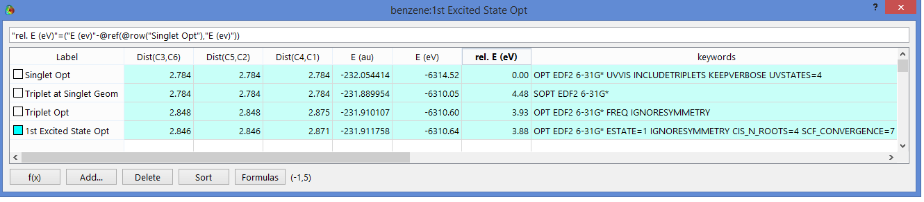
As an example
consider benzene. The ground state was optimized. The HOMO-LUMO gap
of 6.6 eV for this singlet would be a first approximation of the
excited state energy. This molecule is copied+pasted in the
spreadsheet and is submitted as a triplet. This is done twice,
once with a triplet optimization, once at the same singlet geometry.
The energy gain going from singlet to triplet is shown in the
“Rel. E(eV)” column (notice highlighted equation).
The single point energy would be the appropriate number for
fluorescence (vertical excitation), and the triplet optimization
would be for phosphorescence.
 Notice for the triple opt., symmetry is turned off with the
IGNORESYMMETRY keyword and the IR box is checked
(which becomes the FREQ keyword) to ensure one finds the
real triplet minimum.
Any negative frequencies would indicate that symmetry was not
sufficiently broken.
Notice for the triple opt., symmetry is turned off with the
IGNORESYMMETRY keyword and the IR box is checked
(which becomes the FREQ keyword) to ensure one finds the
real triplet minimum.
Any negative frequencies would indicate that symmetry was not
sufficiently broken.
As an example of a different approach/theory,
a UV/Vis calculation was run on the ground-state singlet
(the UVVIS keyword).
Also added were KEEPVERBOSE and INCLUDETRIPLETS,
as mentioned in our help content.
Additionally added was UVSTATES=4 because benzene is a difficult case,
meaning poor convergence. If one examines the verbose output it is
shown that using full TDDFT theory, the excited state energy
(vertical excitation) is 3.88 eV (the TDA approximation gives 4.24 eV).
...TDDFT is probably better ..... needed for other excited states or
singlet->singlet transitions.
We can do optimizations at the TDDFT level,
as shown in the final row. These can be very slow
(prohibitively slow for DFT functionals where analytical
gradients are not available, as is the case for EDF2).
Back to Top
What does the UV/Vis calculation do?
The UV/Vis spectra is calculated by running a single point CIS
calculation (or TD-DFT calculation for DFT methods)
after the main wave function has been calculated.
In CIS theory, the absorption energies
are the difference between the HF ground state and CIS
excited state energies. A reference for Spartan's CIS implementation:
J.B. Foresman, M. Head-Gordon, J.A. Pople,
M.J. Frisch, J. Phys. Chem. (1992), 96, 135.
For DFT calculations, excited states are obtained using the
time-dependent density functional theory (TD-DFT) approach to
generate excited states from excitations of the ground state
molecular orbitals.
The Tamm-Dancoff approximation (TDA) is also available to speed
up the calculations:
E. Runge, U. Gross, Phys. Rev. Lett. (1984) 961533]
A CIS-like Tamm-Dancoff approximation
[S. Hirata, M. Head-Gordon, Chem. Phys. Lett. (1999) 302 375S.
Hirata, M. Head-Gordon, Chem. Phys. Lett. (1999) 314 291
This calculation is similar to the CIS calculation, and most
keywords controlling the excited state CIS calculation are used
in the TDDFT calculation.
A UV/Vis calculation is done, by default, whenever a single-point
excited state calculation is specified. If one needs to modify the
UV/Vis calculation, (other than with the
UVSTATES keyword)
a single point excited state
calculation must be performed, using the keywords described
below.
Back to Top
How can I control an excited state calculation?
See the keyword section on CIS/TDDFT for
relevant keywords. If you want a geometry
optimization for something other than the first excited state,
use the ESTATE=n keyword to choose a different
excited state. (Note that when you hit the "Enter" key the
ESTATE keyword disappears and the n appears where
the "First Excited" in the first line of the calculations dialogue.
Often you may want the first excited singlet state, which may
or may not be the actual first excited state. To limit the
search of possible excited states to singlets you can type in
the keyword CIS_TRIPLETS=FALSE.
Back to Top
What is the difference between the "first excited state"
and "ground state doublet"?
Assuming that the real ground state is a singlet, and the first
excited state is not a triplet, these both refer to the same
electronic state. A difference exists in how Spartan calculates
these; excited state calculations use either CIS or TDFT
methods while ground state calculations use HF or DFT methods.
The later may not be as accurate, but are much faster,
especially in the context of geometry optimizations.
It is also possible that the first excited state is another
singlet, and not a triplet. If in doubt you can do an energy
calculations with the "UV/Vis Spectrum" and the
INCLUDETRIPLETS
keyword to examine all the excited states. Note that the
description of singlet/triplet is found in the verbose output so
you will need to add the KEEPVBOSE keyword. Graphically,
the intensity of the singlet to triplet will be very small.
Back to Top
How can I read the verbose output of
excited state calculations?
It should be noted that information on each excitation can be
found in the verbose output. The notation:
D(10)->V(2) refers to
the excitation of an electron from the 10-th doubly occupied MO
to the 2nd virtual MO. Often, an excitation will take
contributions from multiple molecular orbitals.
The Transition dipole moment and oscillator strength are also
printed. The oscillator strengths are used by Spartan to
graphically display the UV/Vis spectrum. To convert the
oscillator strength to absorbance, we divide by
4.319x10⁻⁷. Usually the log (base 10) of the
absorbance is used to display the spectrum.
By default only pairs of filled/unfilled orbitals which
have amplitudes larger than 0.15.
To see more components you can use the
CIS_AMPL_PRINT=1 keyword
to see (nearly) all of the components.
The sum of the square of all components will sum to 1.0.
Back to Top
How is the NMR spectrum calculated
Spartan supports calculation of chemical shifts for closed shell
(systems with zero unpaired electrons), based on the
Kussmann Ochsenfeld linear scaling algorithm using
"gauge-including atomic orbitals" (GIAOs):
- C. Ochsenfeld, J. Kussmann, F. Koziol, Angew. Chem., 116,
4585, (2004).
- F. London, J. Phys. Radium, 8, 397, (1937)
- K. Wolinski, J. F. Hinton, P. Pulay, J. Am. Chem. Soc.,
112, 8251, (1990).
This scheme has been proven to be reliable and accurate for many applications, see
- T. Helgaker, M. Jaszunski and K. Ruud, Chem. Rev., 99, 293, (1990).
- C. Ochsenfeld and M. Head{Gordon, Chem. Phys. Lett., 270, 399, (1997).
- S. P. Brown, T. Schaller, U. P. Seelbach, F. Koziol,
C. Ochsenfeld, F.-G. Klarner, H. W. Spiess,
Angew. Chem. Int. Ed., 40, 717, (2001).
- C. Ochsenfeld, F. Koziol, S. P. Brown, T. Schaller,
U. P. Seelbach, F.-G. Klarner, Solid
StateNucl. Magn. Reson., 22, 128, (2002).
- C. Ochsenfeld, J. Kussmann, F. Koziol, Angew. Chem., 116,
4585, (2004).
Chemical shifts are given in parts-per-million (ppm) relative
to the appropriate standard (nitromethane for nitrogen,
fluorotrichloromethane for fluorine, and TMS for hydrogen,
carbon and silicon). These relative shifts are available for
most common DFT functionals and basis sets.
One can edit the "NMR_References.spp" file found in the
Spartan shipping directory to add new standards.
Spartan can also apply systematic corrections to the Carbon
NMR depending on the nearby chemical environment. These are
referred to as "corrected shifts" in Spartan.
Back to Top
How is the H-H coupling spectrum calculated?
By default we use modified Karplus equations to predict hydrogen
coupling constants:
- "Vuister and Bax", 1993a and "Wang and Bax 1996" for
amide bonds.
- "Haasnoot, de Leeuw and Altona (1980)" for sp3-sp3 3JHH linkages
- When 2JHH couplings are calculated, we have a few
empirical values from table 4.6 (pg. 151) "Organic Structure
Analysis 2nd ed." P.Crews, J.Rodriguez, M.Jaspers.
Recently we have also added a feature to calculate scalar coupling
constants (J-coupling) from first principles.
For "non range-seperated" DFT functionals
(i.e. B3LYP works, wB97X-D doesn't) we can calculate coupling
constants (J) by directly calculating the indirect coupling tensor.
This can be done from the Calculations dialogue,
if one specifies Coupling Contacts as Calculated (Fermi Contact).
This will utilize the PCJ-0 basis set. This is usually great for 3+ bond coupling,
and "good enough" for 2 bond coupling.
Larger basis sets (PCJ-1 or PCJ-2) are available,
but take significantly longer (and may have difficulty converging for large systems)
and are typically not worth it for 2 and 3 bond coupling.
To run the "Full" ISSC calculation using the FC, SD, PSO and DSO
contributions
you can specify this via the keywords:
JISSC=FULL,PCJ-1 or JISSC=FULL,PCJ-2.
Back to Top
NMR calculations are having difficulty
converging. What can I do?
The NMR calculation has its own set of SCF convergence issues.
Usually the default parameters are good enough to get reasonable
answers, but at times you may need to change these to get
difficult systems to converge. The first thing to do is to
make sure the integrals are more accurate than usual by typing
the CONVERGE keyword in the
Options line of the Calculations dialog.
If you continue to have difficulty you will have to adjust some
of the internal parameters to the multi-step SCF logic. The most
common problem areerrors with "level-2" iterations. By default
this fails after 75 steps. This can be increased with the
D_SCF_MAX_2= keyword. A list of other NMR related
keywords can be found in the
keyword table below.
Back to Top
What is the DP4 score
In Spartan we report a DP4 score for NMR comparison with experiment. This
refers to the DP4. Note that in this context DP4
refers to the statstical measure, not one of the (many) DP4 recipies.
In the following there are 3 descriptions for varying levels of detail:
Back to Top
What is the score used to rank alignments?
The score used for alignment is designed to be 1 for a perfect
fit and 0 for a terrible fit. For a system with N centers:
score = 1 - U/N
U = sum[i=1,N; Gi(ri-roi)]
'ri' is the i'th center of the trial molecule, and
'roi' is the corresponding center of the template
molecule.
G is a function which behaves like the usual Hookean
spring for small values.
(~(ri-roi)2)
but approaches 1 as the difference
in distances (ri-roi) goes to infinity
G =
(1/3)*[ (ri-roi)/Ri]2
G = (1/3)*{3 -
3[(ri-roi)/Ri]-2 +
[(ri-roi)/Ri]-4 }
The second equation is used when
(ri-roi)/Ri
is greater than 1.0.
The normalizing Ri is (3/5) of the
van-der-Wall radii for atoms, and for CFD's is the radii given
in the property panel when a CFD is selected.
The distinguishing feature of this function when compared to a
simple RMSD type function
(ri-roi)2
is that in the case where most of the centers will line up
exactly, but only 1 is nowhere near matching, the latter
center will adversely affect the alignment of the former
centers. As an example, let's try to map the H2 molecule onto a
template of the Br2 molecule with
RBr set
anomalously small, say 1/10 of an angstrom. The 'best' (and
only) minima found by the RMSD function is the H2 molecule
centered symmetrically at the center of the Br2 molecule. The
score we use would find an off-center minima with one
hydrogen directly on one Bromine, and the other Hydrogen near
the center of the Br2 molecule.
When aligning two separate sets of centers, a number of
alignments are examined. It should be noted that the
6-dimensional translation/rotation space of the above function
can have many local minima, or alignments. These are minimized
and examined, and the best one is returned. Also,
a second score is used internally: 'the number of 'matched
centers'. This score closely matches the reported score, but
any alignment in which some center-pairings do not line up with
Ri are rejected, prior to comparing actual
score values.
Back to Top
What is the score used to rank molecules in
the similarity module
The score used in alignment
is used in the
similarity task. The similarity task is more time consuming
than alignment in that similarity will look at multiple ways of
matching two molecules using different atom mappings and/or
pharmacophores, and can look at multiple conformations stored in
"Similarity Libraries". This score can be displayed in the
resulting spreadsheet by typing
Sim. Score=
into a column header of the spreadsheet.
Back to Top
What are the units used in Spartan?
- Geometries
Cartesian coordinates are typically given in Ångstroms (Å), but are also
available in nanometers (nm) and atomic units (au).
Bond distances are typically given in Å,
but are also available in nm and au. Bond angles and dihedral
angles are given in degrees (°).
Surface areas are typically given in Å2
and volumes in Å3, but are also
available in nm2 (nm3) and au2 (au3).
1 Å = 0.1 nm = 1.889762 au
- Energies, Heats of Formation and Strain Energies
Total energies from Hartree-Fock, density functional and MP2 calculations
are typically given in au, but are also available in
kcal/mol, kJ/mol and electron volts (eV).
Heats of formation from semi-empirical calculations and thermochemical recipes
are typically given in kJ/mol, but are also available in au, kcal/mol and eV.
Strain energies from molecular mechanics calculations are
typically given in kJ/mol, but are also available in au, kcal/mol and eV.
- Orbital Energies
Orbital energies from Hartree-Fock, density functional and
MP2 calculations are typically given in ev,
but are also available in kcal/mol, kJ/mol and au.
Orbital energies
from semi-empirical calculations are
typically given in eV, but are also available in kcal/mol,
kJ/mol and au.
- Energy Conversions
Energy Conversionsa
| |
au |
kcal/mol |
kJ/mol |
eV |
| 1 au |
- |
6.275x10² |
2.625x10³ |
2.721x101 |
| 1 kcal/mol |
1.593x10⁻³ |
- |
4.184 |
4.337x10⁻² |
| 1 kJ/mol |
3.809x10⁻⁴ |
2.390x10⁻¹ |
- |
1.036x10⁻² |
| 1 eV |
3.675x10⁻² |
2.306x101 |
96.485 |
- |
- Graphical Properties
Electron densities and spin densities are given in electrons/au3.
Dipole moments are given in debyes.
Electrostatic potentials are given in kJ/mol.
- Other Properties
Atomic charges are given in electrons.
Vibrational frequencies are given in wavenumbers
(cm-1).
Back to Top
What are the conversion factors used in Spartan?
Below are some commonly used conversion factors:
 Energy:
   1 au (Hartree)=       me*e^4/h-bar^2
                 =       4.3597482(26) 10^-18  J              *
	         =       4.35974381(34)10^-18  J      (1998 CODATA)
                 =     627.510                 kcal/mol
                       627.5095602             kcal/mol       *
                       627.50947093            kcal/mol (1998 CODATA [new Na])
   1 ev          =       1.60217733(49) 10^-19 J              *
   1 ev          =     96.485                  kJ/mol
   4.184 J       =       1                     Calorie (a constant)
   1 kT (T=300K) ~       2.495                 kJ

 Entropy:
   1 e.u.        =       4.184                 J/mol*K
                 =       1                     cal/mol*K

 Pressure:
   1 kbar        =       10^8                  Pa
                 =    986.923267               atm
   1 atm         =    101.325                  k Pa (exact)   *

 Length:
   1 A           =       10^-10                m
                 =       1.8897269             au   (old value)
                 =       1.889725988579        au
   1 au (Bohr)   =       h-bar^2/(me*e^2)
                 =       0.529177249(24)       A              *
	         =       0.5291772083(19)      A (new CODATA 1998)

 Mass:
   1 AMU         =       1.6605402(10)  10^-27 Kg (Atomic Mass Unit)
                 =       1.66053873(13) 10^-27 Kg (new CODATA 1998)
   Mass C12      =      12.0                   AMU
                 =      12.0                   g/mol/Na
   1 mn          =       1.67492716(13) 10^-27 Kg (Mass of neutron)
   1 mp          =       1.67262158(13) 10^-27 Kg (Mass of proton)
                         1.007276470(12)       AMU
   1 me          =       9.1034897(54) 10^-31 Kg (Mass of electron)
                         9.10938188(72)10^-31 Kg
                         0.5109906(15)         Mev
 Wavenumber:
   1 cm^-1       =       2.9979 10^-10 s^-1
                 =       0.29979 THz
   2.19474.7 cm-1=       1 Hartree^-1/2 Bohr^-1 AMU^-1/2

 Wavelength:             (for light = 1/Wavenumber)
                 =       h*c/Energy      (for light)
   1 nm          =       1239.837/ev     (ie. homo-lumo gap)
                 =       1.9166 10^-4/kJ (Na in energy)

 Charge:
   1 au          =       1                e
                 =       1.602 10^-19     C
                 =       2.452 10^-18     esu*cm

 Dipole moment:
   1 debye(D)    =       3.336e-30        C*m
                 =       0.20824          e*A
   1 au          =       8.479e-30        C*m
                 =       2.542e-18        esu*cm
                 =       2.542            D

 Polarizability:
   1 au          =       14.83e-30        m^3
                 =       14.83            A^3

 Moment-of-Inertia:
   I  cm^-1      =       60.1997601/I[ AMU*bhors^2 ]
   I  cm^-1      =       16.8576522/I[ AMU*A^2     ]
*In places where multiple values are listed for a given
conversion, the first is the approximation used in Spartan,
the second is the 'exact' value (as of 1973,
1986 or 1998).
Return to Top
What are the fundamental constants used in Spartan?
Below are some important constants used in quantum chemistry:
Speed of Light   :    c :  2.99792458    10^10   cm/s      * (exact)
Avogadro's Num.  :   Na :  6.0221367(36) 10^23             *
                     Na :  6.02214199(47)10^23             (1998 CODATA)
Gas Constant     :    R :  8.314510(70)          J/K/mol   *
                      R :  8.314472(15)          J/K/mol   (1998 CODATA)
Boltzmann const. :    k :  1.380658(12)  10^-23  J/K       *
			   1.3806503(24) 10^-23  J/K       (1998 CODATA)
Planck's const.  :    h :  6.626075(40)  10^-34  J s       *
                           6.62606876(52)10^-34  J s       (1998 CODATA)
                           6.62607015    10^-34  J s       (exact definition 2018)
fine-structure   : alpha:  1/137.0359895(61)
                           7.297352533(27) 10^-3           (1998 CODATA)
*In places where multiple values are listed for a given
conversion the first is the approximation used in Spartan,
the second is the 'exact' value
(as of 1973, 1986 or 1998).
Back to Top
New research has resulted in the
measurement of a more accurate value for an important constant.
Will Spartan reflect this change?
No. Data sets using the older constants have been generated
for more than 30 years. To make sure newer versions maintain
backward compatibility we continue to use the older values for
these fundamental constants and conversion factors. Even though
each new digit is an important scientific achievement,
the increased precision is well beneath the noise present in
the chemical measurements Spartan deals with.
Back to Top
Support@wavefun.com